Scikit-learn 简介：使用感知器

Scikit-learn 的名字源于 SciKit (SciPy Toolkit)，即 SciPy 的第三方扩展工具包。经过历年的发展，Scikit-learn 已成为最流行的机器学习库之一。本文以 Iris 数据集的分类为例，对其进行简介。

如官方网站所介绍，以下是 scikit-learn 的特征：

• 简单高效的数据挖掘和数据分析工具
• 可供任何人使用，可在任何环境中重复使用
• 基于 NumPy，SciPy，以及 matplotlib
• 开放源码，可用作商业用途 (需遵循 BSD 许可证)

关于 scikit-learn 的安装，请参照这份文档。

数据导入

从 scikit-learn 加载 Iris 数据集，其中第三列表示花瓣长度 petal length，第四列表示花瓣宽度 petal width。这些类已经转换为整数标签，其中 0 = 山鸢尾 Iris-Setosa，1 = 变色鸢尾 Iris-Versicolor，2 = 维吉尼亚鸢尾 Iris-Verginica。

from sklearn import datasets
import numpy as np

iris = datasets.load_iris()
X = iris.data[:, [2, 3]]
y = iris.target

print("Class labels:", np.unique(y))  # output: Class labels: [0 1 2]

预处理

通过函数 sklearn.model_selection.train_test_split 将 150 个数据集分为 70% 的训练集和 30% 的测试集：

from sklearn.model_selection import train_test_split

X_train, X_test, y_train, y_test = train_test_split(
    X, y, test_size=0.3, random_state=1, stratify=y
)

这里 stratify=y 表示按照标签值将数据集划分，划分后训练集和测试集的标签具有相同的比例，可以用 np.bincount 打印其中每类标签的个数：

print("Labels counts in y:", np.bincount(y))  # output: Labels counts in y: [50 50 50]
print(
    "Labels counts in y_train:", np.bincount(y_train)
)  # output: Labels counts in y_train: [35 35 35]
print(
    "Labels counts in y_test:", np.bincount(y_test)
)  # output: Labels counts in y_test: [15 15 15]

通过函数 sklearn.preprocessing.StandardScaler 对特征进行标准化：

from sklearn.preprocessing import StandardScaler

sc = StandardScaler()
sc.fit(X_train)
X_train_std = sc.transform(X_train)
X_test_std = sc.transform(X_test)

模型训练

使用神经元模型 sklearn.linear_model.Perceptron，对训练集进行训练 fit：

from sklearn.linear_model import Perceptron

ppn = Perceptron(max_iter=40, eta0=0.1, random_state=0)
ppn.fit(X_train_std, y_train)

模型评估

训练完成后，对测试集进行预测 predict，并打印出其中错误预测的样本数量：

y_pred = ppn.predict(X_test_std)
print(
    "Misclassified samples: %d" % (y_test != y_pred).sum()
)  # output: Misclassified samples: 3

训练准确率可以通过 sklearn.metrics.accuracy_score 得到：

from sklearn.metrics import accuracy_score

print("Accuracy: %.2f" % accuracy_score(y_test, y_pred))  # output: Accuracy: 0.93

scikit-learn 中的每种分类函数都有计算准确率的方法 score，执行时会计算 accuracy_score 并返回，输出结果相同：

print("Accuracy: %.2f" % ppn.score(X_test_std, y_test))  # output: Accuracy: 0.93

绘制分类边界

对算法训练过程进行绘图：

from matplotlib.colors import ListedColormap
import matplotlib.pyplot as plt


def plot_decision_regions(X, y, classifier, test_idx=None, resolution=0.02):
    markers = ("s", "x", "o", "^", "v")
    colors = ("red", "blue", "lightgreen", "gray", "cyan")
    cmap = ListedColormap(colors[: len(np.unique(y))])

    x1_min, x1_max = X[:, 0].min() - 1, X[:, 0].max() + 1
    x2_min, x2_max = X[:, 1].min() - 1, X[:, 1].max() + 1
    xx1, xx2 = np.meshgrid(
        np.arange(x1_min, x1_max, resolution), np.arange(x2_min, x2_max, resolution)
    )
    Z = classifier.predict(np.array([xx1.ravel(), xx2.ravel()]).T)
    Z = Z.reshape(xx1.shape)
    plt.contourf(xx1, xx2, Z, alpha=0.3, cmap=cmap)
    plt.xlim(xx1.min(), xx1.max())
    plt.ylim(xx2.min(), xx2.max())
    for idx, cl in enumerate(np.unique(y)):
        plt.scatter(
            x=X[y == cl, 0],
            y=X[y == cl, 1],
            alpha=0.8,
            c=colors[idx],
            marker=markers[idx],
            label=cl,
            edgecolor="black",
        )

    if test_idx:
        X_test, y_test = X[test_idx, :], y[test_idx]
        plt.scatter(
            X_test[:, 0],
            X_test[:, 1],
            c="",
            edgecolor="black",
            alpha=1.0,
            linewidth=1,
            marker="o",
            s=100,
            label="test set",
        )


X_combined_std = np.vstack((X_train_std, X_test_std))
y_combined = np.hstack((y_train, y_test))
plot_decision_regions(
    X=X_combined_std, y=y_combined, classifier=ppn, test_idx=range(105, 150)
)
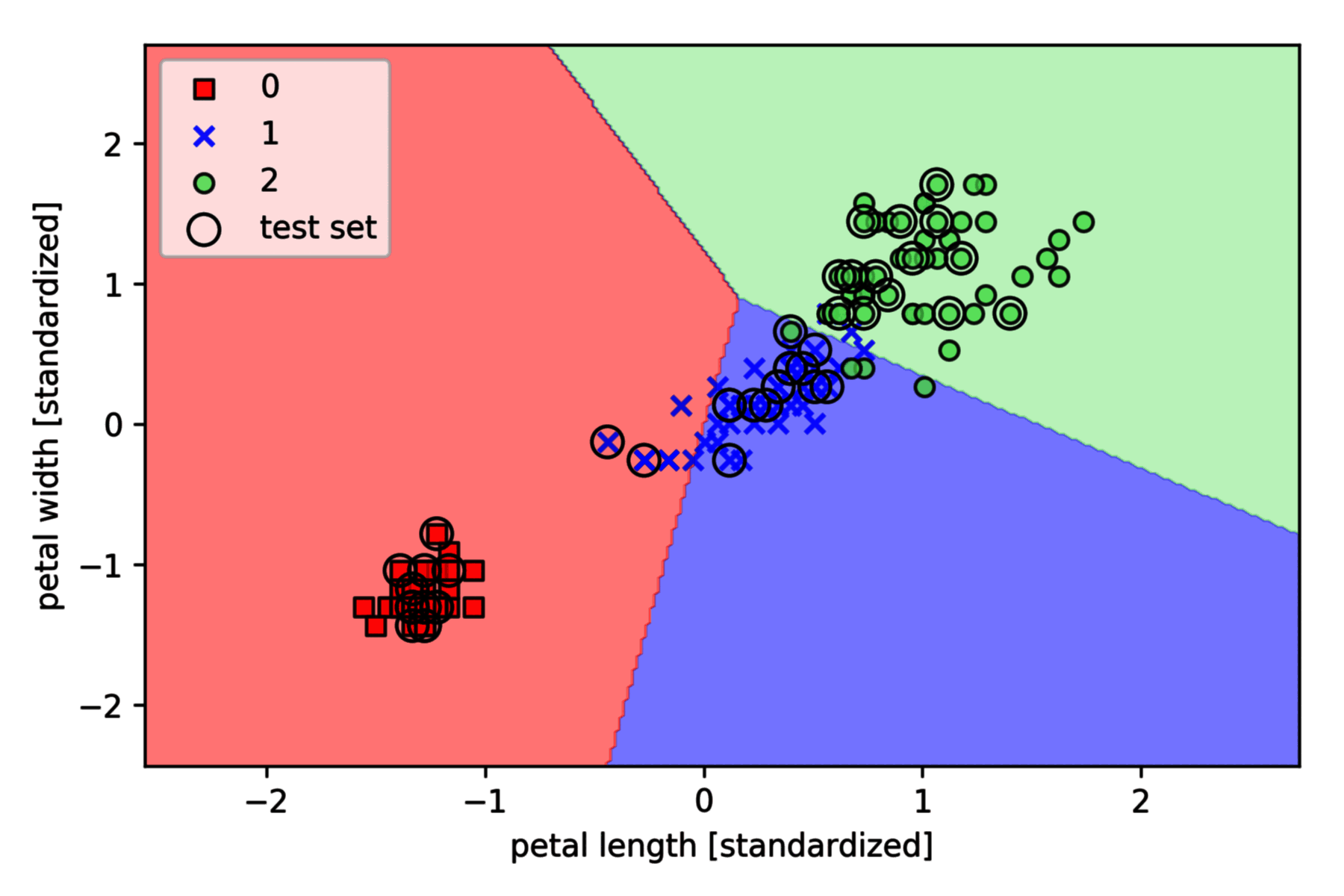
plt.xlabel("petal length [standardized]")
plt.ylabel("petal width [standardized]")
plt.legend(loc="upper left")
plt.show()

绘制边界如下，其中测试集用黑色圆圈标出：