NumPy 快速入门
NumPy 是用于 Python 中多维数组计算的软件库。
本文部分内容翻译自斯坦福大学文档 CS231n - Python NumPy Tutorial。
什么是 NumPy
NumPy 是 Python 中科学计算的基础包。它是一个 Python 库,提供多维数组对象、各种派生对象 (例如数组和矩阵) 以及各种用于快速数组操作的例程,包括数学、逻辑、形状操作、排序、选择、I/O、离散傅里叶变换、基本线性代数、基本统计运算、随机模拟等等。
NumPy 包的核心是 ndarray 对象。它封装了同构数据类型的 n 维数组,许多操作在编译代码中执行以提高性能。NumPy 数组和标准 Python 序列之间有几个重要的区别:
- 与 Python 列表 (可以动态增长) 不同,NumPy 数组在创建时大小是固定的。更改 ndarray 的大小将创建一个新数组并删除原始数组。
- NumPy 数组中的元素都必须具有相同的数据类型,因此在内存中的大小也相同。例外:可以拥有 (Python,包括 NumPy) 对象的数组,从而允许不同大小元素的数组。
- NumPy 数组有助于对大量数据进行高级数学和其他类型的运算。通常,与使用 Python 的内置序列相比,此类操作的执行效率更高,并且代码更少。
越来越多的基于 Python 的科学和数学包正在使用 NumPy 数组;尽管这些通常支持 Python 序列输入,但它们在处理之前将此类输入转换为 NumPy 数组,并且通常输出 NumPy 数组。换句话说,为了有效地使用当今大部分 (甚至是大多数) 基于 Python 的科学/数学软件,仅仅知道如何使用 Python 的内置序列类型是不够的 - 还需要知道如何使用 NumPy 数组。
关于序列大小和速度的问题在科学计算中尤为重要。作为一个简单的示例,考虑将一维序列中的每个元素与相同长度的另一个序列中的相应元素相乘的情况。如果数据存储在两个 Python 列表 a 和 b 中,我们可以迭代每个元素:
c = []
for i in range(len(a)):
    c.append(a[i] * b[i])
这会产生正确的答案,但如果 a 和 b 各自包含数百万个数字,我们将为 Python 中的循环效率低下付出代价。我们可以通过编写 C 语言更快地完成相同的任务 (为了清楚起见,我们忽略了变量声明和初始化、内存分配等)
for (i = 0; i < rows; i++) {
  c[i] = a[i]*b[i];
}
这节省了解释 Python 代码和操作 Python 对象所涉及的所有开销,但代价是牺牲了从 Python 编码中获得的好处。此外,所需的编码工作随着数据维度的增加而增加。例如,在二维数组的情况下,C 代码 (如前所述) 扩展为
for (i = 0; i < rows; i++) {
  for (j = 0; j < columns; j++) {
    c[i][j] = a[i][j]*b[i][j];
  }
}
NumPy 为我们提供了两全其美的功能:当涉及 ndarray 时,逐元素操作是“默认模式”,但逐元素操作可以通过预编译的 C 代码快速执行。在 NumPy 中可以用
c = a * b
执行前面示例的操作,速度接近 C 语言,同时代码简单,符合我们基于 Python 的期望。
为什么 NumPy 很快?
矢量化的代码没有任何显式循环、索引等 - 当然,这些事情实际上是在优化的预编译 C 代码中被处理了。矢量化代码具有许多优点,其中包括:
- 矢量化代码更简洁,更容易阅读
- 更少的代码行通常意味着更少的错误
- 代码更类似于标准数学符号 (通常更容易正确编码数学结构)
- 矢量化会产生更多符合 Python 风格的代码;如果没有矢量化,我们的代码将充斥着低效且难以阅读的
for循环
使用 Numpy
Numpy 是 Python 中科学计算的核心库。它提供了一个高性能的多维数组对象,以及使用这些数组的工具。
数组
Numpy 的核心功能是 ndarray (即 n-dimensional array,多维数组) 数据结构。这是一个表示多维度、同质并且固定大小的数组对象。维数是数组的秩 rank;数组的形状 shape 是一个整数元组,表示沿着每个维度的数组大小。
我们可以从嵌套的 Python 列表初始化 Numpy 数组,并使用方括号来访问元素:
import numpy as np

a = np.array([1, 2, 3])  # Create a rank 1 array
print type(a)            # Prints "<type 'numpy.ndarray'>"
print a.shape            # Prints "(3,)"
print a[0], a[1], a[2]   # Prints "1 2 3"
a[0] = 5                 # Change an element of the array
print a                  # Prints "[5, 2, 3]"

b = np.array([[1,2,3],[4,5,6]])   # Create a rank 2 array
print b.shape                     # Prints "(2, 3)"
print b[0, 0], b[0, 1], b[1, 0]   # Prints "1 2 4"
Numpy 还提供许多创建数组的函数:
import numpy as np

a = np.zeros((2,2))  # Create an array of all zeros
print a              # Prints "[[ 0.  0.]
                     #          [ 0.  0.]]"

b = np.ones((1,2))   # Create an array of all ones
print b              # Prints "[[ 1.  1.]]"

c = np.full((2,2), 7) # Create a constant array
print c               # Prints "[[ 7.  7.]
                      #          [ 7.  7.]]"

d = np.eye(2)        # Create a 2x2 identity matrix
print d              # Prints "[[ 1.  0.]
                     #          [ 0.  1.]]"

e = np.random.random((2,2)) # Create an array filled with random values
print e                     # Might print "[[ 0.91940167  0.08143941]
                            #               [ 0.68744134  0.87236687]]"
你可以在这份文档中阅读关于数组创建的其他方法。
数组索引
Numpy 提供了多种索引到数组的方法。
切片:与 Python 列表类似,可以对 Numpy 数组进行切片。由于数组可能是多维的,因此必须为数组的每个维度指定一个切片:
import numpy as np

# Create the following rank 2 array with shape (3, 4)
# [[ 1  2  3  4]
#  [ 5  6  7  8]
#  [ 9 10 11 12]]
a = np.array([[1,2,3,4], [5,6,7,8], [9,10,11,12]])

# Use slicing to pull out the subarray consisting of the first 2 rows
# and columns 1 and 2; b is the following array of shape (2, 2):
# [[2 3]
#  [6 7]]
b = a[:2, 1:3]

# A slice of an array is a view into the same data, so modifying it
# will modify the original array.
print a[0, 1]   # Prints "2"
b[0, 0] = 77    # b[0, 0] is the same piece of data as a[0, 1]
print a[0, 1]   # Prints "77"
你还可以将整数索引与片段索引进行混合。但是,这样做会产生比原始数组更低的数组:
import numpy as np

# Create the following rank 2 array with shape (3, 4)
# [[ 1  2  3  4]
#  [ 5  6  7  8]
#  [ 9 10 11 12]]
a = np.array([[1,2,3,4], [5,6,7,8], [9,10,11,12]])

# Two ways of accessing the data in the middle row of the array.
# Mixing integer indexing with slices yields an array of lower rank,
# while using only slices yields an array of the same rank as the
# original array:
row_r1 = a[1, :]    # Rank 1 view of the second row of a
row_r2 = a[1:2, :]  # Rank 2 view of the second row of a
print row_r1, row_r1.shape  # Prints "[5 6 7 8] (4,)"
print row_r2, row_r2.shape  # Prints "[[5 6 7 8]] (1, 4)"

# We can make the same distinction when accessing columns of an array:
col_r1 = a[:, 1]
col_r2 = a[:, 1:2]
print col_r1, col_r1.shape  # Prints "[ 2  6 10] (3,)"
print col_r2, col_r2.shape  # Prints "[[ 2]
                            #          [ 6]
                            #          [10]] (3, 1)"
整数数组索引:当你使用切片索引到 Numpy 数组时,生成的数组视图将始终是原始数组的子数组。相反,整数数组索引允许你使用另一个数组的数据来构造任意数组。例如:
import numpy as np

a = np.array([[1,2], [3, 4], [5, 6]])

# An example of integer array indexing.
# The returned array will have shape (3,) and
print a[[0, 1, 2], [0, 1, 0]]  # Prints "[1 4 5]"

# The above example of integer array indexing is equivalent to this:
print np.array([a[0, 0], a[1, 1], a[2, 0]])  # Prints "[1 4 5]"

# When using integer array indexing, you can reuse the same
# element from the source array:
print a[[0, 0], [1, 1]]  # Prints "[2 2]"

# Equivalent to the previous integer array indexing example
print np.array([a[0, 1], a[0, 1]])  # Prints "[2 2]"
一个有用的整数数组索引技巧,是从矩阵的每一行中选择一个元素:
import numpy as np

# Create a new array from which we will select elements
a = np.array([[1,2,3], [4,5,6], [7,8,9], [10, 11, 12]])

print a  # prints "array([[ 1,  2,  3],
         #                [ 4,  5,  6],
         #                [ 7,  8,  9],
         #                [10, 11, 12]])"

# Create an array of indices
b = np.array([0, 2, 0, 1])

# Select one element from each row of a using the indices in b
print a[np.arange(4), b]  # Prints "[ 1  6  7 11]"

# Mutate one element from each row of a using the indices in b
a[np.arange(4), b] += 10

print a  # prints "array([[11,  2,  3],
         #                [ 4,  5, 16],
         #                [17,  8,  9],
         #                [10, 21, 12]])
布尔数组索引:布尔数组索引可以让你选择数组的任意元素。通常,这种类型的索引用于选择满足某些条件的数组的元素。例如:
import numpy as np

a = np.array([[1,2], [3, 4], [5, 6]])

bool_idx = (a > 2)  # Find the elements of a that are bigger than 2;
                    # this returns a numpy array of Booleans of the same
                    # shape as a, where each slot of bool_idx tells
                    # whether that element of a is > 2.

print bool_idx      # Prints "[[False False]
                    #          [ True  True]
                    #          [ True  True]]"

# We use boolean array indexing to construct a rank 1 array
# consisting of the elements of a corresponding to the True values
# of bool_idx
print a[bool_idx]  # Prints "[3 4 5 6]"

# We can do all of the above in a single concise statement:
print a[a > 2]     # Prints "[3 4 5 6]"
为了简洁起见,我们省略了很多有关 Numpy 数组索引的细节;如果你想了解更多,请阅读这份文档。
数据类型
每个 Numpy 数组都是相同类型元素的网格。Numpy 提供了大量可用于构造数组的数值数据类型。创建数组时,Numpy 会尝试猜测数据类型,但构造数组的函数通常还包含一个可选参数来显式指定数据类型。下面是一个例子:
import numpy as np

x = np.array([1, 2])  # Let numpy choose the datatype
print(x.dtype)  # Prints "int64"

x = np.array([1.0, 2.0])  # Let numpy choose the datatype
print(x.dtype)  # Prints "float64"

x = np.array([1, 2], dtype=np.int64)  # Force a particular datatype
print(x.dtype)  # Prints "int64"
你可以在这份文档中查看 Numpy 支持的数据类型。
数组计算
基本的数学函数在数组上按元素运算,并且可以作为运算符重载和 numpy 模块中的函数使用:
import numpy as np

x = np.array([[1,2],[3,4]], dtype=np.float64)
y = np.array([[5,6],[7,8]], dtype=np.float64)

# Elementwise sum; both produce the array
# [[ 6.0  8.0]
#  [10.0 12.0]]
print x + y
print np.add(x, y)

# Elementwise difference; both produce the array
# [[-4.0 -4.0]
#  [-4.0 -4.0]]
print x - y
print np.subtract(x, y)

# Elementwise product; both produce the array
# [[ 5.0 12.0]
#  [21.0 32.0]]
print x * y
print np.multiply(x, y)

# Elementwise division; both produce the array
# [[ 0.2         0.33333333]
#  [ 0.42857143  0.5       ]]
print x / y
print np.divide(x, y)

# Elementwise square root; produces the array
# [[ 1.          1.41421356]
#  [ 1.73205081  2.        ]]
print np.sqrt(x)
请注意,* 是元素乘法,而不是矩阵乘法。如需使用矩阵乘法,请使用函数 dot。dot 可用作 Numpy 模块中的函数,也可用作数组对象的实例方法:
import numpy as np

x = np.array([[1,2],[3,4]])
y = np.array([[5,6],[7,8]])

v = np.array([9,10])
w = np.array([11, 12])

# Inner product of vectors; both produce 219
print v.dot(w)
print np.dot(v, w)

# Matrix / vector product; both produce the rank 1 array [29 67]
print x.dot(v)
print np.dot(x, v)

# Matrix / matrix product; both produce the rank 2 array
# [[19 22]
#  [43 50]]
print x.dot(y)
print np.dot(x, y)
Numpy 提供了许多有用的矩阵计算函数;其中最重要的函数之一是 sum:
import numpy as np

x = np.array([[1,2],[3,4]])

print np.sum(x)  # Compute sum of all elements; prints "10"
print np.sum(x, axis=0)  # Compute sum of each column; prints "[4 6]"
print np.sum(x, axis=1)  # Compute sum of each row; prints "[3 7]"
你可以在这份文档中找到 numpy 提供的数学函数完整列表。
除了使用数组计算数学函数之外,我们经常需要重新整形或以其他方式处理数组中的数据。这种类型的操作的最简单的例子是转置矩阵;要转置矩阵,只需使用数组对象的 T 属性:
import numpy as np

x = np.array([[1,2], [3,4]])
print x    # Prints "[[1 2]
           #          [3 4]]"
print x.T  # Prints "[[1 3]
           #          [2 4]]"

# Note that taking the transpose of a rank 1 array does nothing:
v = np.array([1,2,3])
print v    # Prints "[1 2 3]"
print v.T  # Prints "[1 2 3]"
Numpy 提供了更多的功能来操作数组;你可以在这份文档中看到完整列表。
广播
广播是一种强大的机制,允许 Numpy 在执行算术运算时使用不同形状的数组。通常我们有一个更小的数组和一个更大的数组,我们想要使用较小的数组多次来对较大的数组执行一些操作。
例如,假设我们要为矩阵的每一行添加一个常量向量。我们可以这样做:
import numpy as np

# We will add the vector v to each row of the matrix x,
# storing the result in the matrix y
x = np.array([[1,2,3], [4,5,6], [7,8,9], [10, 11, 12]])
v = np.array([1, 0, 1])
y = np.empty_like(x)   # Create an empty matrix with the same shape as x

# Add the vector v to each row of the matrix x with an explicit loop
for i in range(4):
    y[i, :] = x[i, :] + v

# Now y is the following
# [[ 2  2  4]
#  [ 5  5  7]
#  [ 8  8 10]
#  [11 11 13]]
print y
这种方法是可以的;然而,当矩阵 x 非常大时,Python 循环可能会运行很长时间。实际上,将向量 v 添加到矩阵 x 的每一行,等价于通过创建垂直堆叠 v 的矩阵 vv,然后执行 x 和 vv 的元素求和。我们可以这样实现这个方法:
import numpy as np

# We will add the vector v to each row of the matrix x,
# storing the result in the matrix y
x = np.array([[1,2,3], [4,5,6], [7,8,9], [10, 11, 12]])
v = np.array([1, 0, 1])
vv = np.tile(v, (4, 1))  # Stack 4 copies of v on top of each other
print vv                 # Prints "[[1 0 1]
                         #          [1 0 1]
                         #          [1 0 1]
                         #          [1 0 1]]"
y = x + vv  # Add x and vv elementwise
print y  # Prints "[[ 2  2  4
         #          [ 5  5  7]
         #          [ 8  8 10]
         #          [11 11 13]]"
Numpy 广播允许我们在不创建 v 的多个副本的情况下执行这个计算。以上情况下,我们可以使用广播:
import numpy as np

# We will add the vector v to each row of the matrix x,
# storing the result in the matrix y
x = np.array([[1,2,3], [4,5,6], [7,8,9], [10, 11, 12]])
v = np.array([1, 0, 1])
y = x + v  # Add v to each row of x using broadcasting
print y  # Prints "[[ 2  2  4]
         #          [ 5  5  7]
         #          [ 8  8 10]
         #          [11 11 13]]"
即使 x 具有形状 (4, 3) 且 v 具有形状 (3,),行 y = x + v 可以正常执行;工作原理是由于广播,v 仿佛有形状 (4, 3),其中每行都是 v 的副本,然后按元素进行求和。
两个数组间的广播遵循以下规则:
- 如果阵列不具有相同的秩,则对较小秩的阵列进行预处理,直到两个形状都具有相同的长度。
- 如果两个数组在某一维度的大小相等,或者其中一个数组在该维度的大小为 1,则称两个数组在这个维度上兼容。
- 如果两个数组在所有维度上都兼容,则可以进行广播。
- 广播后,每个数组形状等同于较大的数组形状。
- 如果在某一维度,其中一个数组大小等于 1 并且另一个数组大小大于 1,则前者沿着此维度复制自身。
支持广播的函数被称为通用函数。你可以在这份文档中找到所有通用函数的列表。
以下是广播的一些应用:
import numpy as np

# Compute outer product of vectors
v = np.array([1,2,3])  # v has shape (3,)
w = np.array([4,5])    # w has shape (2,)
# To compute an outer product, we first reshape v to be a column
# vector of shape (3, 1); we can then broadcast it against w to yield
# an output of shape (3, 2), which is the outer product of v and w:
# [[ 4  5]
#  [ 8 10]
#  [12 15]]
print np.reshape(v, (3, 1)) * w

# Add a vector to each row of a matrix
x = np.array([[1,2,3], [4,5,6]])
# x has shape (2, 3) and v has shape (3,) so they broadcast to (2, 3),
# giving the following matrix:
# [[2 4 6]
#  [5 7 9]]
print x + v

# Add a vector to each column of a matrix
# x has shape (2, 3) and w has shape (2,).
# If we transpose x then it has shape (3, 2) and can be broadcast
# against w to yield a result of shape (3, 2); transposing this result
# yields the final result of shape (2, 3) which is the matrix x with
# the vector w added to each column. Gives the following matrix:
# [[ 5  6  7]
#  [ 9 10 11]]
print (x.T + w).T
# Another solution is to reshape w to be a column vector of shape (2, 1);
# we can then broadcast it directly against x to produce the same
# output.
print x + np.reshape(w, (2, 1))

# Multiply a matrix by a constant:
# x has shape (2, 3). NumPy treats scalars as arrays of shape ();
# these can be broadcast together to shape (2, 3), producing the
# following array:
# [[ 2  4  6]
#  [ 8 10 12]]
print x * 2
广播通常会使你的代码更加简洁快捷,因此你应尽可能地使用它。
Numpy 文档
这个简短的概述已经涉及到大部分 Numpy 的重要功能,但仍有许多地方未涉及。查看 Numpy 参考文档以了解更多关于 Numpy 的信息。
Scipy
Numpy 提供了一个高性能的多维数组和基本的工具来计算和操纵这些数组。Scipy 建立在此基础之上,并提供了大量功能,可以运行在 Numpy 数组上,并且可用于不同类型的科学和工程应用。
熟悉 Scipy 的最佳方法是浏览这份文档。
图像操作
Scipy 提供了一些基本功能来处理图像。例如,它具有从磁盘读取图像到 Numpy 数组,将 Numpy 数组写入磁盘作为图像并调整图像大小的功能。下面的示例中展示了这些功能:
from scipy.misc import imread, imsave, imresize

# Read an JPEG image into a numpy array
img = imread('assets/cat.jpg')
print img.dtype, img.shape  # Prints "uint8 (400, 248, 3)"

# We can tint the image by scaling each of the color channels
# by a different scalar constant. The image has shape (400, 248, 3);
# we multiply it by the array [1, 0.95, 0.9] of shape (3,);
# numpy broadcasting means that this leaves the red channel unchanged,
# and multiplies the green and blue channels by 0.95 and 0.9
# respectively.
img_tinted = img * [1, 0.95, 0.9]

# Resize the tinted image to be 300 by 300 pixels.
img_tinted = imresize(img_tinted, (300, 300))

# Write the tinted image back to disk
imsave('assets/cat_tinted.jpg', img_tinted)


点的距离
Scipy 定义了一些有用的函数,用于计算点集合之间的距离。
函数 scipy.spatial.distance.pdist 计算给定单个集合中所有点之间的距离:
import numpy as np
from scipy.spatial.distance import pdist, squareform

# Create the following array where each row is a point in 2D space:
# [[0 1]
#  [1 0]
#  [2 0]]
x = np.array([[0, 1], [1, 0], [2, 0]])
print x

# Compute the Euclidean distance between all rows of x.
# d[i, j] is the Euclidean distance between x[i, :] and x[j, :],
# and d is the following array:
# [[ 0.          1.41421356  2.23606798]
#  [ 1.41421356  0.          1.        ]
#  [ 2.23606798  1.          0.        ]]
d = squareform(pdist(x, 'euclidean'))
print d
你可以在这份文档中阅读有关此功能的所有详细信息。
类似的函数 (scipy.spatial.distance.cdist) 能够计算不同集合内所有点之间的距离;你可以阅读这份文档。
Matplotlib
Matplotlib 是一个绘图库。本节简要介绍了 matplotlib.pyplot 模块,该模块提供了与 MATLAB 类似的绘图系统。
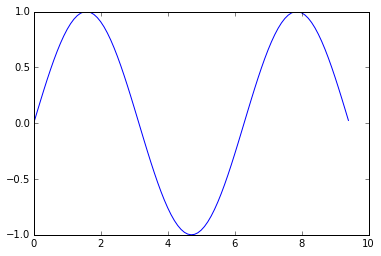
绘图
Matplotlib 中最重要的函数是 plot,它可以绘制二维数据。这是一个简单的例子:
import numpy as np
import matplotlib.pyplot as plt

# Compute the x and y coordinates for points on a sine curve
x = np.arange(0, 3 * np.pi, 0.1)
y = np.sin(x)

# Plot the points using matplotlib
plt.plot(x, y)
plt.show()  # You must call plt.show() to make graphics appear.
运行此代码,会生成以下图形:
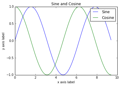
只需一点额外的工作,我们可以轻松地绘制多行,并添加标题,图例和轴标签:
import numpy as np
import matplotlib.pyplot as plt

# Compute the x and y coordinates for points on sine and cosine curves
x = np.arange(0, 3 * np.pi, 0.1)
y_sin = np.sin(x)
y_cos = np.cos(x)

# Plot the points using matplotlib
plt.plot(x, y_sin)
plt.plot(x, y_cos)
plt.xlabel("x axis label")
plt.ylabel("y axis label")
plt.title("Sine and Cosine")
plt.legend(["Sine", "Cosine"])
plt.show()
关于 plot 函数的更多信息,你可以阅读这份文档。
绘制子图
你可以使用 subplot 函数在同一图中绘制不同子图。例如:
import numpy as np
import matplotlib.pyplot as plt

# Compute the x and y coordinates for points on sine and cosine curves
x = np.arange(0, 3 * np.pi, 0.1)
y_sin = np.sin(x)
y_cos = np.cos(x)

# Set up a subplot grid that has height 2 and width 1,
# and set the first such subplot as active.
plt.subplot(2, 1, 1)

# Make the first plot
plt.plot(x, y_sin)
plt.title("Sine")

# Set the second subplot as active, and make the second plot.
plt.subplot(2, 1, 2)
plt.plot(x, y_cos)
plt.title("Cosine")

# Show the figure.
plt.show()
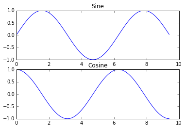
关于 subplot 函数的更多信息,你可以阅读这份文档。
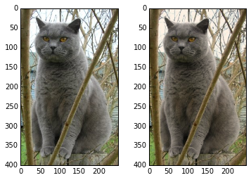
图像
你可以使用 imshow 功能来显示图像。例如:
import numpy as np
from scipy.misc import imread, imresize
import matplotlib.pyplot as plt

img = imread("assets/cat.jpg")
img_tinted = img * [1, 0.95, 0.9]

# Show the original image
plt.subplot(1, 2, 1)
plt.imshow(img)

# Show the tinted image
plt.subplot(1, 2, 2)

# A slight gotcha with imshow is that it might give strange results
# if presented with data that is not uint8. To work around this, we
# explicitly cast the image to uint8 before displaying it.
plt.imshow(np.uint8(img_tinted))
plt.show()