决策树和随机森林

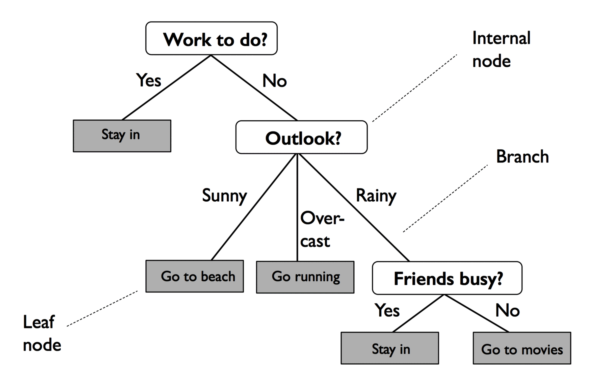
决策树 (Decision Tree) 是一种特殊的树结构，代表的是样本特征与样本标签之间的一种映射关系。

决策树举例如下，分叉路径则代表某个可能的属性值，而终结节点代表最终决策：

信息增益

定义

为了引入决策树分类的算法，先介绍决策树学习中的重要概念：信息增益 (Information Gain)。

这个指标可以衡量分类给数据中带来信息的程度。若分类带来的信息增益越大，就越能减少数据的无序度。

信息增益的表示如下，为父节点和子节点中的不纯度 (Inpurity) 差值：

$$\begin{align} IG(D_p, f) = I(D_p) - \sum_{j=1}^m \cfrac {N_i} {N_p} I(D_j) \end{align}$$

其中 $f$ 代表对应的特征，$D_p$ 和 $D_j$ 分别表示父节点的数据和第 $j$ 个子节点的数据集，$N_p$ 和 $N_i$ 分别表示父节点的数据和第 $j$ 个子节点的样本数量，$I()$ 代表不纯度的函数。

不纯度的计算有以下几种方法：

• 熵 (Entropy)：$I_H(t) = -\sum_{j=1}^c p(i \mid t) \cdot \log_2 p(i \mid t)$
• Gini 不纯度 (Gini Impurity)：$I_G(t) = 1- \sum_{j=1}^c p(i \mid t)^2$
• 分类错误 (Classification Error)：$I_E(t) = 1- \max p(i \mid t)$

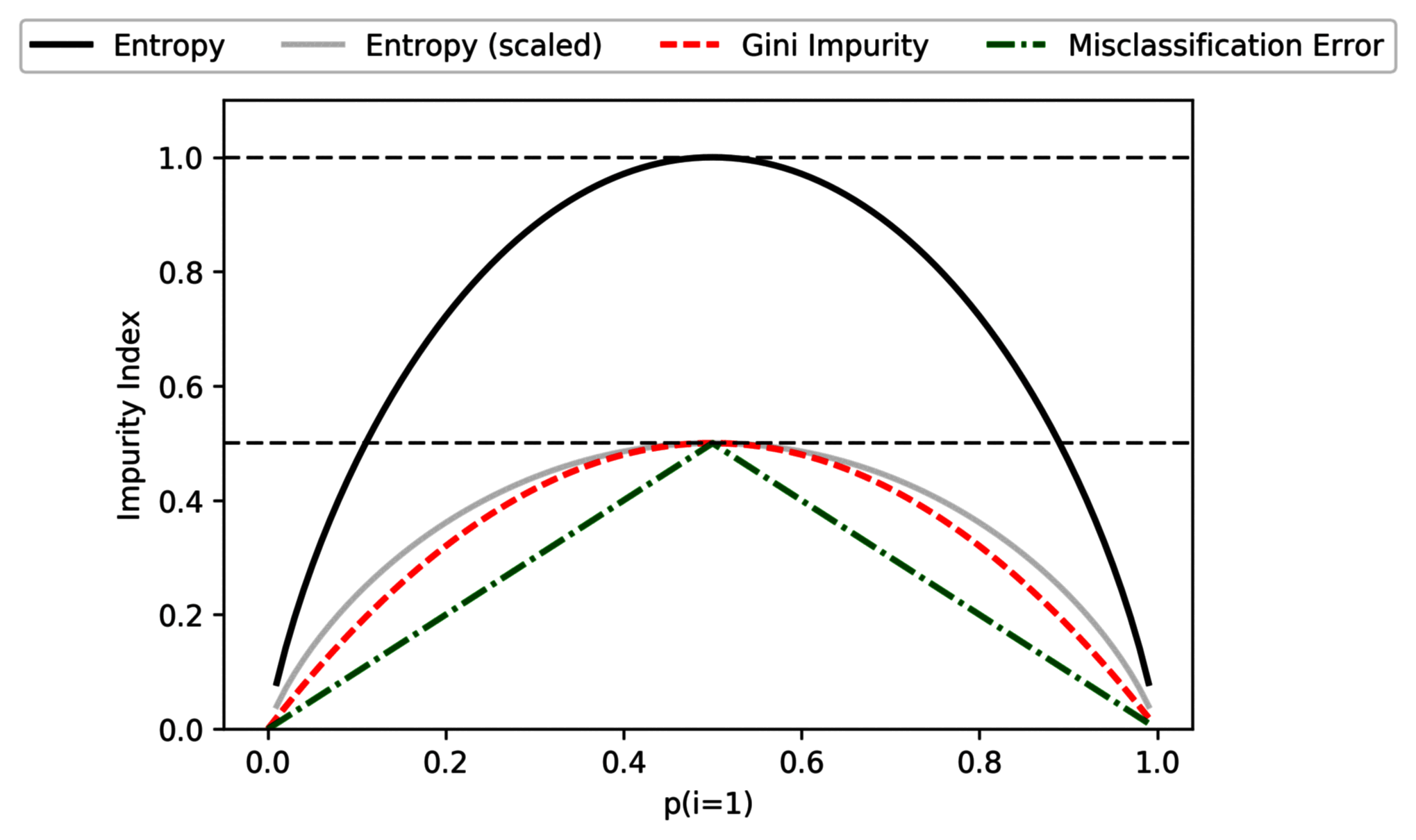
在实际应用中，熵和 Gini 不纯度的结果非常相似，不必纠结于这两个计算标准的选择。而分类错误对节点概率的变化较不敏感，不推荐在决策树增长时使用。

计算示例

以如下决策树演示不纯度的计算，其中 $(a，b)$ 代表节点中所属分类的样本数量。

例如父节点，包含 40 个属于类 1 的样本、40 个属于类 2 的样本；其他节点同理。

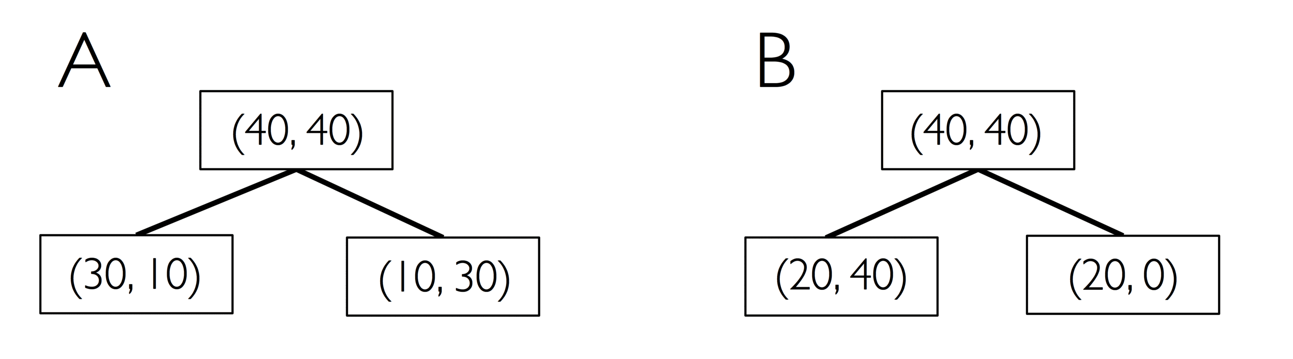
决策树 A 的熵：

$$\begin{align} I_H(D_p) & = -({\cfrac 1 2} \log{\cfrac 1 2} + {\cfrac 1 2} \log{\cfrac 1 2}) = 1 \\ I_H(D_{left}) & = -({\cfrac 3 4} \log{\cfrac 3 4} + {\cfrac 1 4} \log{\cfrac 1 4}) = 0.81 \\ I_H(D_{right}) & = -({\cfrac 1 4} \log{\cfrac 1 4} + {\cfrac 3 4} \log{\cfrac 3 4}) = 0.81 \\ IG_H & = 1 - {\cfrac 1 2} 0.81 - {\cfrac 1 2} 0.81 = 0.19 \end{align}$$

决策树 B 的熵：

$$\begin{align} I_H(D_p) & = -({\cfrac 1 2} \log{\cfrac 1 2} + {\cfrac 1 2} \log{\cfrac 1 2}) = 1 \\ I_H(D_{left}) & = -({\cfrac 1 3} \log{\cfrac 1 3} + {\cfrac 2 3} \log{\cfrac 2 3}) = 0.92 \\ I_H(D_{right}) & = 0 \\ IG_H & = 1 - {\cfrac 3 4} 0.92 - 0 = 0.31 \end{align}$$

决策树 A 的 Gini 不纯度：

$$\begin{align} I_G(D_p) & = 1 - ({\cfrac 1 2})^2 - ({\cfrac 1 2})^2 = \cfrac 1 2 \\ I_G(D_{left}) & = 1 - ({\cfrac 3 4})^2 - ({\cfrac 1 4})^2 = \cfrac 3 8 \\ I_G(D_{right}) & = 1 - ({\cfrac 1 4})^2 - ({\cfrac 3 4})^2 = \cfrac 3 8 \\ IG_G & = 1 - {\cfrac 1 2} \cdot {\cfrac 3 8} - {\cfrac 1 2} \cdot {\cfrac 3 8} = 0.125 \end{align}$$

决策树 B 的 Gini 不纯度：

$$\begin{align} I_G(D_p) & = 1 - ({\cfrac 1 2})^2 - ({\cfrac 1 2})^2 = \cfrac 1 2 \\ I_G(D_{left}) & = 1 - ({\cfrac 2 3})^2 - ({\cfrac 1 3})^2 = \cfrac 4 9 \\ I_G(D_{right}) & = 1 - 1^2 - 0^2 = 0 \\ IG_G & = \cfrac 1 2 - {\cfrac 3 4} \cdot {\cfrac 4 9} - 0 = 0.167 \end{align}$$

决策树 A 的分类错误：

$$\begin{align} I_E(D_p) & = 1 - {\cfrac 1 2} = \cfrac 1 2 \\ I_E(D_{left}) & = 1 - {\cfrac 3 4} = \cfrac 1 4 \\ I_E(D_{right}) & = 1 - {\cfrac 3 4} = \cfrac 1 4 \\ IG_E & = {\cfrac 1 2} - {\cfrac 1 2} \cdot {\cfrac 1 4} - {\cfrac 1 2} \cdot {\cfrac 1 4} = 0.25 \end{align}$$

决策树 B 的分类错误：

$$\begin{align} I_E(D_p) & = 1 - {\cfrac 1 2} = \cfrac 1 2 \\ I_E(D_{left}) & = 1 - {\cfrac 1 3} = \cfrac 1 3 \\ I_E(D_{right}) & = 1 - 1 = 0 \\ IG_E & = {\cfrac 1 2} - {\cfrac 3 4} \cdot {\cfrac 1 3} - 0 = 0.25 \end{align}$$

为了更直观的比较三种信息增益计算方法的差异，对平均分布 $[0,1]$ 的样本应用并绘图：

import matplotlib.pyplot as plt
import numpy as np


def gini(p):
    return (p) * (1 - (p)) + (1 - p) * (1 - (1 - p))


def entropy(p):
    return -p * np.log2(p) - (1 - p) * np.log2((1 - p))


def error(p):
    return 1 - np.max([p, 1 - p])


x = np.arange(0.0, 1.0, 0.01)
ent = [entropy(p) if p != 0 else None for p in x]
sc_ent = [e * 0.5 if e else None for e in ent]
err = [error(i) for i in x]

ax = plt.subplot(111)
for (
    i,
    lab,
    ls,
    c,
) in zip(
    [ent, sc_ent, gini(x), err],
    ["Entropy", "Entropy (scaled)", "Gini Impurity", "Misclassification Error"],
    ["-", "-", "--", "-."],
    ["black", "lightgray", "red", "green", "cyan"],
):
    line = ax.plot(x, i, label=lab, linestyle=ls, lw=2, color=c)
ax.legend(
    loc="upper center", bbox_to_anchor=(0.5, 1.15), ncol=5, fancybox=True, shadow=False
)
ax.axhline(y=0.5, linewidth=1, color="k", linestyle="--")
ax.axhline(y=1.0, linewidth=1, color="k", linestyle="--")

plt.ylim([0, 1.1])
plt.xlabel("p(i=1)")
plt.ylabel("Impurity Index")
plt.show()

决策树

代码实现

决策树分类的思想是，从树根开始将特征上的数据分割成最大的信息增益，然后在子节点重复这个拆分过程。

在实践中，这可能会导致一个有很多节点的很深的树，很容易导致过度拟合。因此通常要通过设置树的最大深度限制来修剪树。

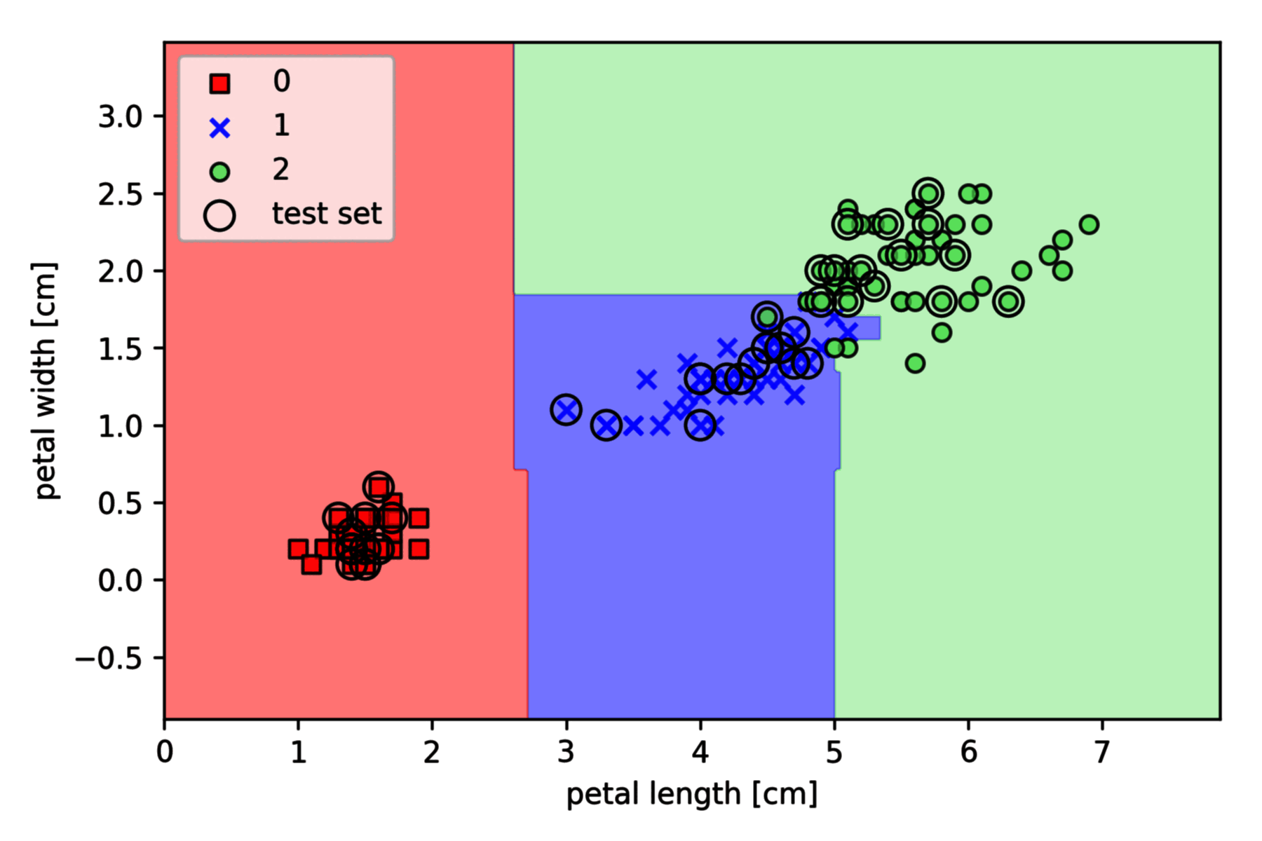
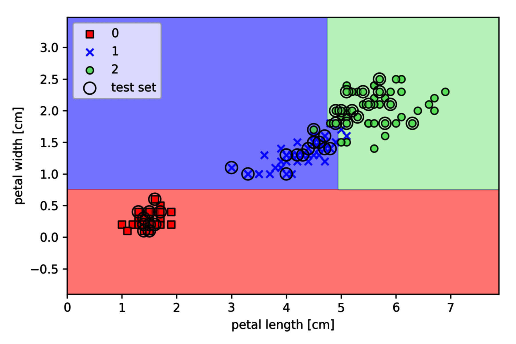
以 Iris 数据集为例，基于 Scikit-learn 的实现如下 (其中决策边界绘制函数 plot_decision_regions 请参见之前的文章)：

import matplotlib.pyplot as plt
import numpy as np
from sklearn import datasets
from sklearn.model_selection import train_test_split
from sklearn.tree import DecisionTreeClassifier

iris = datasets.load_iris()
X = iris.data[:, [2, 3]]
y = iris.target
X_train, X_test, y_train, y_test = train_test_split(
    X, y, test_size=0.3, random_state=1, stratify=y
)

tree = DecisionTreeClassifier(criterion="gini", max_depth=4, random_state=1)
tree.fit(X_train, y_train)

X_combined = np.vstack((X_train, X_test))
y_combined = np.hstack((y_train, y_test))
plot_decision_regions(X_combined, y_combined, classifier=tree, test_idx=range(105, 150))
plt.xlabel("petal length [standardized]")
plt.ylabel("petal width [standardized]")
plt.legend(loc="upper left")
plt.show()

Graphviz 绘图

Windows 下的 Graphviz 需要：

1. 下载并安装 Graphviz Windows 安装包 graphviz-2.xx.msi
2. 将 C:\Program Files (x86)\Graphviz2.xx\bin\; 添加到环境变量 Path (计算机——属性——高级系统设置——环境变量)
3. Pip 安装软件包：pip install pydotplus graphviz pyparsing

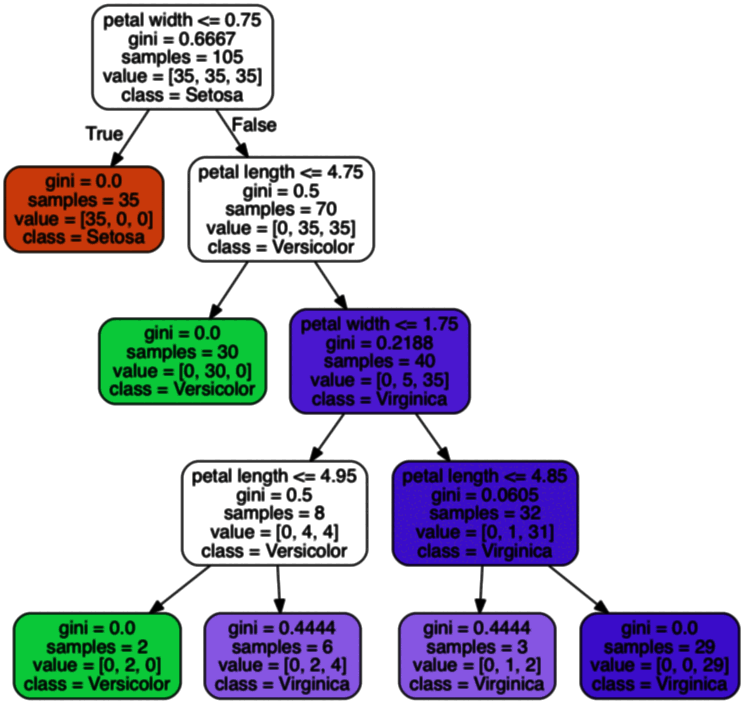
对上节生成的 tree 进行绘图：

from pydotplus import graph_from_dot_data
from sklearn.tree import export_graphviz

dot_data = export_graphviz(
    tree,
    filled=True,
    rounded=True,
    class_names=["Setosa", "Versicolor", "Virginica"],
    feature_names=["petal length", "petal width"],
    out_file=None,
)
graph = graph_from_dot_data(dot_data)
graph.write_png("tree.png")

随机森林

随机森林是一个包含多个决策树的分类器，并且其输出的分类标签是由每个树的的分类标签的众数而定。

1. 从已知的样本集合 (样本数 $M$，特征数 $N$) 中，有放回地随机取 $n$ 个 bootstrap 样本 ($n < N$)。
2. 对取得的 bootstrap 的样本生成决策树：a。无放回地随机选择其中 $m$ 个特征 ($m << M$)。b。根据目标函数提供的最佳分割特征 (如最大化信息增益) 来分割节点。
3. 重复步骤 1-2 若干次数。
4. 汇总每棵树的预测标签，把其中数量最多的作为随机森林的分类标签。

import matplotlib.pyplot as plt
import numpy as np
from sklearn import datasets
from sklearn.model_selection import train_test_split
from sklearn.ensemble import RandomForestClassifier

iris = datasets.load_iris()
X = iris.data[:, [2, 3]]
y = iris.target
X_train, X_test, y_train, y_test = train_test_split(
    X, y, test_size=0.3, random_state=1, stratify=y
)

forest = RandomForestClassifier(
    criterion="gini", n_estimators=25, random_state=1, n_jobs=2
)
forest.fit(X_train, y_train)

X_combined = np.vstack((X_train, X_test))
y_combined = np.hstack((y_train, y_test))
plot_decision_regions(
    X_combined, y_combined, classifier=forest, test_idx=range(105, 150)
)
plt.xlabel("petal length [standardized]")
plt.ylabel("petal width [standardized]")
plt.legend(loc="upper left")
plt.show()

上面通过 n_estimators 参数从 25 个决策树中训练了一个随机森林，并使用 Gini 不纯度作为分割节点的标准。n_jobs 参数表示可以使用计算机的多个核心 (这里是两个核心) 来并行化训练。